12 most popular Excel’s formulas

Excel’s top 12 most popular formulas with examples

Excel has over 475 formulas in its Functions Library, from simple mathematics to very complex statistical, logical, and engineering tasks such as IF statements (one of our perennial favorite stories); AND, OR, NOT functions; COUNT, AVERAGE, and MIN/MAX.

The basic functions covered below are the top 12 most popular formulas in Excel. To help you learn, we've also provided a spreadsheet with all the formula examples we cover below.

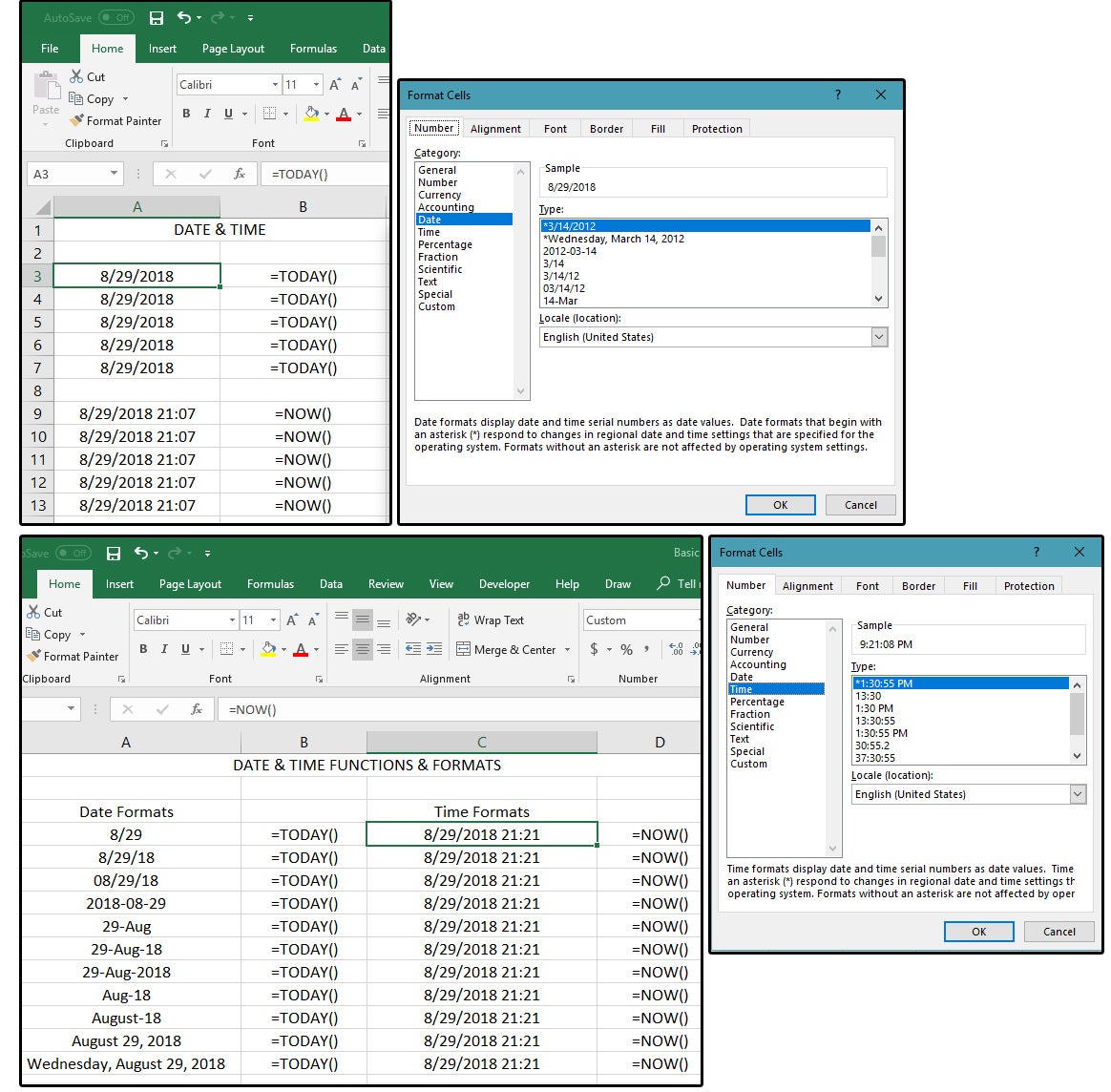
1. TODAY/NOW

There are 24 Date and Time functions listed on the drop-down menu under Formulas > Date & Time: 11 Date formats, 10 Time formats, and as many user-defined custom formats you can create. The TODAY function reveals the current month, day, and year; while the NOW function reveals the current month, day, year, and time of day. This is a handy function if you’re one of those individuals who always forgets to date your work.

1. Enter the following formula in cell A1: =TODAY() and press Enter.
2. Next, type over that function in A1 with =NOW().
   IMPORTANT NOTE: Why type over? In order for these two formulas to work properly, they must be entered in the Home cell, that is, A1, otherwise, they won’t update automatically when the spreadsheet recalculates. Press Shift- F9 to calculate/recalculate the active spreadsheet only, or press F9 for the entire workbook.After you enter one of these functions in A1, you can then reformat the Date and Time or use the system default. The default format for the TODAY function is 8/29/18, and the default for NOW is 8/29/18 21:57. If these don’t work for you, change them.
3. Position your cursor on the Date or Time you want changed and choose Home > Format > Format Cells.
4. In the Format Cells dialog window, choose Date (or Time) from the Category panel under the Number tab.
5. Scroll through the list of Date/Time formats in the Type dialog pane and select the format that best fits your project.

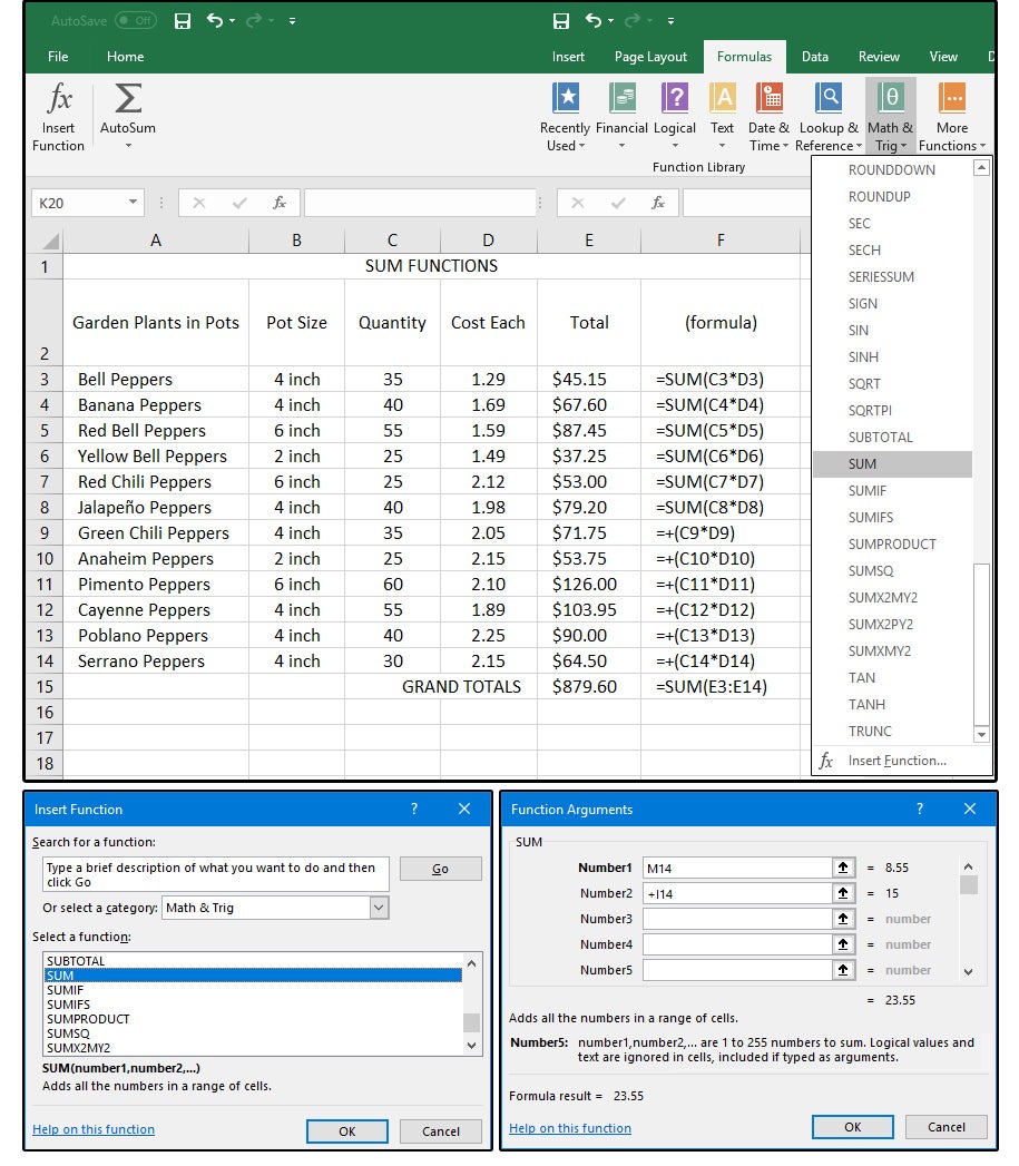
2. SUM functions

Probably the most frequently used function in Excel (or any other spreadsheet program), =SUM does just that: It sums a column, row, or range of numbers—but it doesn’t just sum. It also subtracts, multiplies, divides, and uses any of the comparison operators to return a result of 1 (true) or 0 (false).
You can also get the same results just using the plus (+) sign in place of the function SUM. For example, both of these formulas produce the same answer: =SUM(J7*9) and =+(J7*9). In the spreadsheet graphic below, notice that cells E3 through E8 use the SUM function, while cells E9 through E9 through E14 use the plus (+) sign and the results are the same.
You can enter the SUM function (or + sign) manually or select it from the Ribbon menu under Formulas > Math & Trig (button), then choose from the drop-down list; or choose (from the Ribbon menu) Formulas > Insert Function, then scroll down the list and select it from there.
If you just want to add a single column of numbers, position your cursor in the cell at the bottom of that column, click the AutoSum button > SUM, and press Enter. Excel frames the column of numbers in green borders and displays the formula in the current cell.

The problem comes when the range of numbers you need to calculate gets complicated with multiple calculation operators over multiple cellsFor example: =SUM(H1+I1*J1-M1*J1. Remember your high school math? If the numbers inside the formula are not grouped properly, the answer will be wrong. Notice the screenshot below (figure 2).
Enter the following column headers in H2 through P2 (use Alt+ Enter to stack headers in a single cell): Daily Earnings, Plus Bonuses, Times Days Worked, Gross Pay, (formula), Minus Meals at $9.00 per day, Total Monthly Earnings, Formula, and Comment.
NOTE: The formula columns are FYI only and provide no intrinsic value to the spreadsheet. They just “display” the formula for your benefit (so you can see the syntax of each formula used).
For this exercise, you can enter the same values in H3:11, I3:11, and J3:11, with or without the blank rows in between (again, added for easier viewing). Complete as follows: $86.00, $20.00, 22.0 workdays, and the rest are formulas. Note that as we build each formula, we are combining the steps, eventually, into a single formula.
We start out with three separate formulas. The first is to add the Daily earnings, plus Bonuses, multiplied by the number of days worked in a month, which equals Gross Pay: =SUM(H3+I3*J3) in cell K3. Notice that the answer is $526.00. That just doesn’t look right.
Use your calculator to check the formulas to ensure they’re correct BEFORE you copy them to the rest of the cells in the column.
The formula in K3 is wrong. It requires grouping the numbers according to the order of calculation using commas or parentheses.
Note the corrected formula in cell K4: =SUM(H4+I4)*J4. Check your numbers again (with your calculator) and note that this formula is correct. The correct answer is $2,332.00.
The second formula (in M4) is =SUM(J4*9) multiplies the workdays (22) times $9.00, the cost of meals per day. The correct answer is $198.00.

1. The third formula (in N4) calculates the monthly earnings minus the meals: =SUM(K4-M4); answer is $2,134.00.
2. In the next group (H6:N8), the formulas in M6:M8 remain the same: =SUM(J7*9), etc.—again that’s the number of workdays times the cost of meals. But the formulas in column K are eliminated and then combined with the formulas in column M: =SUM(H7+I7)*J7-M7. Note that the syntax (the structure or layout of the formula) is correct in cells N7 and N8, but incorrect in N6.
3. The next group (H10:H11) combines the formulas in column M with the formulas in column N: =SUM(H11+I11)*J11-(M11*J11)—note that the formula in N10 is incorrect. By combining these formulas into one, you can eliminate columns K and L.
4. Also, instead of “hardcoding” the price of the meals (as shown in M3:M4 and M6:M8), you can now change the price of the meals in column M (M10:M11) when inflation dictates an increase instead of changing the formula.

3. RAND function

The RAND function is really simple and traditionally used for statistical analysis, cryptography, gaming, gambling, and probability theory, among dozens of other things. In Excel, the RAND function generates a random number between 0 and 1. Note; however, that every time you enter new data and press the Enter key, the list of random numbers you just created changes. If you need to maintain your random numbers lists, you must format the cells as values.

1. Enter the function =RAND() in columns A3 through A14. Select that column and press Ctrl+C (for copy) or click the Copy button under the Home tab and choose Copy from the drop-down menu. Move your cursor to cell B3 and select Home > Paste > Paste Special. Click the Values button from the Paste Special dialog window, then click OK.
2. Now the list contains values instead of functions, so it will not change. Notice (in the formula bar) that the random numbers have 15 digits after the decimal (Excel defaults to 9), which you can change, if necessary (as displayed in cell F3). Just click the Increase Decimal button in the Number group under the Home tab.
3. If you prefer to work with whole numbers, enter this formula in cell F3: =INT(RAND()*999) and you get a 3-digit random number. Copy the formula down through F12, then add another '9' to the string to add another digit to your random number—e.g., four nines equal four digits, five nines equal five digits. Again, you must copy the list and Paste as Values to maintain a static list.

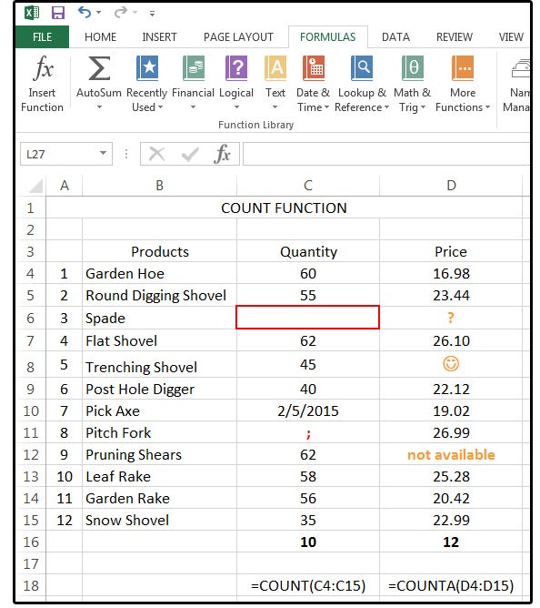
4. COUNT functions

Use the COUNT function to count the number of numeric values in a range of cells; for example: C4:C15 contains the quantity of garden tools Mr. McGregor needs to order for his shop. Note that the answer is 10 (out of 12), because the COUNT function does not include blank cells. However, if you enter a zero, a numeric code, or a date, Excel counts it as an “occupied” cell and includes it in its answer.
Enter 10 numbers into column C (Quantity). Replace one number with a space (or a tap on the spacebar), then replace another number with a semicolon, and then enter a date into cell C7.
Enter this formula at the bottom of the number list (C16): =COUNT(C4:C15). The answer is 10 (out of 12) because Excel counted all the numbers and the date, but ignored the blank cell (containing the space) and the punctuation in cell C8.
Use the COUNTA function if you want to include numeric values, logical or error values, text, a space (from the spacebar), punctuation, symbols, or any other character on your keyboard.

1. Enter 12 dollar amounts into column D (Price). Replace one cell with a question mark, another cell with a symbol, and another cell with some text.
2. Enter this formula in D16: =COUNTA(C4:C15). The answer is 12 (out of 12) because Excel included all the “non-numeric” values and characters.
3. Notice that row 18 (C and D) displays the actual formulas that are in C and D 16.

5. AVERAGE function

Most everyone knows that an average is determined by adding all the values in a list, then dividing by the number of values listed; e.g., 4+5+3=12/3=4, which is the average. You can use the SUM function and add the division all in one formula, or you can just use the AVERAGE function. The syntax is: =AVERAGE(range).
1. Enter some numbers in column A. Enter the AVERAGE function at the bottom of the list: =AVERAGE(A4:A13) and note the answer (in our case) is 53. You can verify your answer with the SUM function; that is: =SUM(A4:A13/10) = 53.
2. Next enter some more numbers in column C but, this time, add some text to one cell, punctuation to another, and a space to another. Enter the same formula: =AVERAGE(A4:A15), and note the answer is 78. To verify, enter the SUM formula omitting the cells that contain non-numeric characters:
Cells that contain text, logical values, punctuation, or empty cells are disregarded; but cells with the zeros (as a number, but not as text) are included. A text zero would have an apostrophe in front of the zero, which you cannot see in the cell, but is visible in the Formula Bar.
IMPORTANT NOTE: If you’re importing huge databases from a mainframe or an outside, external source, sometimes the numbers export as text. How can you know if a number is really text? Generally, text is left-justified and numbers are right-justified but, because everyone formats their spreadsheets for aesthetics now, that method is unreliable. Another option is to scroll quickly through a long list of imported numbers and watch the Formula Bar. If you see apostrophes before any of the numbers, those entries are text. Last, look for the green triangle in the top left corner of the cell. Unless the previous owner of the spreadsheet instructed Excel to ignore this error, then the contents of the cell are text.
If the values are text, you must convert them to numbers immediately. To do this, move down to the first number in the list that’s actually text. Highlight the range of text that’s impersonating numbers. Right-click the yellow warning sign that’s left of the first text cell in the range. Click Convert to Number from the pop-up list, and it’s done.

6. MIN/MAX functions

Use the MIN function to find the smallest number in a range of values, and the MAX function to find the highest. The syntax for these functions are: =MIN(range); =MAX(range) where range equals the list of numbers you’re calculating.
Common uses of this function are; for example, find the highest/lowest grade in a classroom; the highest/lowest sales dollars in a store; the highest/lowest batting averages of your favorite baseball team; and so on.
Some would ask, why not just sort the data? You could, but every time the numbers changed, you’d have to re-sort. And, if you’re sorting multiple columns/fields with a lot of records/rows, the sort option could get cumbersome.
The MIN/MAX functions remain the same regardless of the changes in the data, even if you add more rows (as long as you add the rows using the Insert > Row feature within the existing range--that is, above the cell that contains the formula).
Enter some numbers in column A4:A11, then enter this formula in A13: =MIN(A4:A11) and this formula in A14: =MAN(A4:A11).
NOTE: The MIN/MAX functions disregard empty cells, TRUE/FALSE answers, text, text impersonating numbers, symbols, and punctuation.

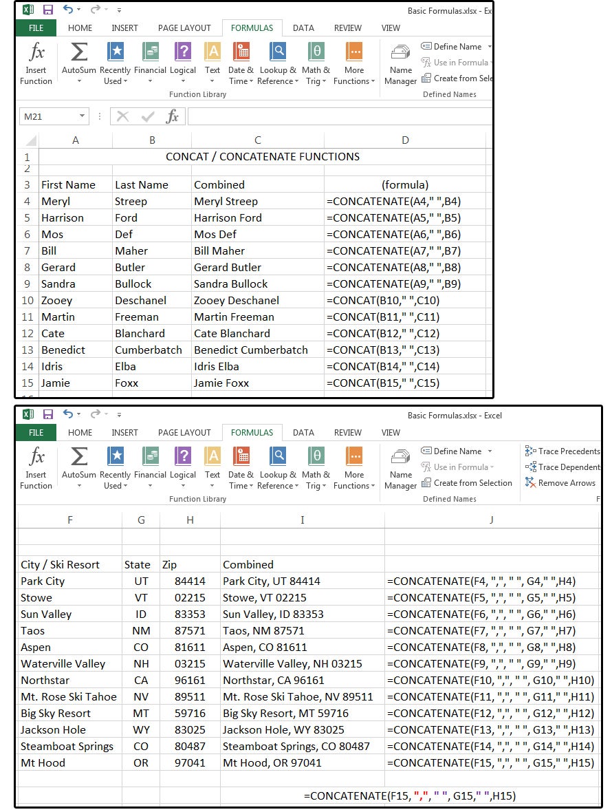
7. CONCAT/CONCATENATE

The functions CONCAT and CONCATENATE do the same thing: They both combine multiple cells, ranges, or strings of data into one cell. The most common use of this function is to combine first and last name into one cell or join the city, state, and ZIP code into one cell.
NOTE: CONCAT replaced CONCATENATE in Excel 2016, but both functions are still available. Note that CONCAT appears only under Formulas > Text and Formulas > Insert Function > Category > Text, but both CONCAT and CONCATENATE appear under Formulas > Insert Function > Category > All.
Enter some first names in column A and last names in column B. Enter the following formula in column C: =CONCATENATE(A4,” “,B4) or =CONCAT(B4,” “,C4), then copy the formula down. What are the double quotes for? See Note below #2.
2. Enter a few cities (or ski resorts) in column F, states in column G, and ZIP codes in column H. Enter the following formula in column I: =CONCATENATE(F4, “,”, “ “, G4,” “,H4).
NOTE: If you want a space between the first and last name, you must enter that space inside quotation marks in your formula. The same thing is true for punctuation, such as a comma between city and state. In the following formula the “,” (quote comma quote—in red) tells Excel to insert a comma between the data in F15 (city) and the data in G15 (state). The “ “ (quote space quote—in purple) adds a space after the comma between F15 (city) and G15 (state) and another space between G15 (state) and H15 (zip code).
=CONCATENATE(F15, ”,”, ” “, G15, ” “,H15).

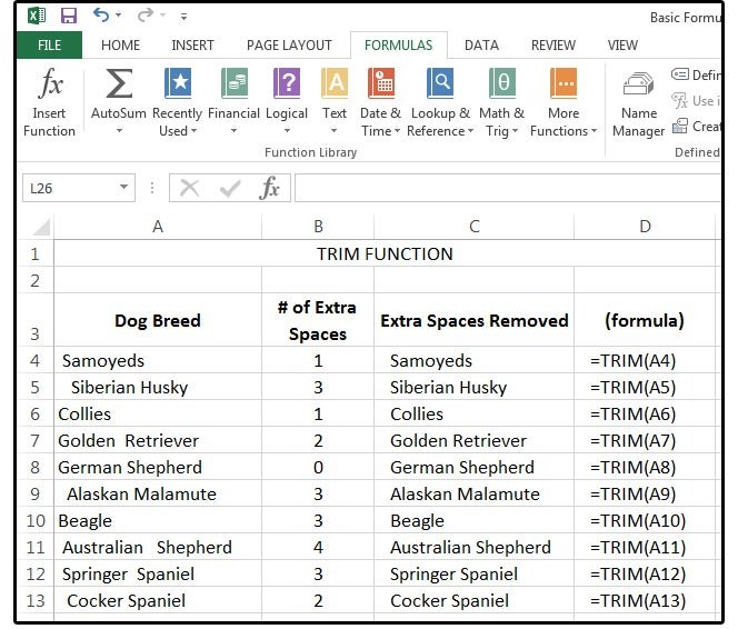
8. TRIM

This function removes extra (or padded) spaces that infect your data as a result of user error, downloading data from an external source such as the Internet, or importing data from another computer system. And you don’t have to “tell Excel” where the spaces are located in the string of text in each cell; it recognizes the extra spaces and removes them. Note; however, that it will not remove a space in the middle of a word. The syntax is simple: =TRIM(cell address).

1. Enter some data in column A. Add some spaces before, after, and in the middle of multiple words, then enter the following formula in cell A4: =TRIM(A4).
2. Copy the formula down. It’s that easy!

NOTE: There is one case where this function does not work, and that's with a non-breaking space character used in webpages. The decimal value is 160, and the HTML code is &nbsp. You can remove this character using a combination of TRIM, CLEAN, and SUBSTITUTE.

9. UPPER/LOWER/PROPER

Another easy group, these functions convert text in a cell or range of cells to uppercase, lowercase or proper case. Proper case is first letter in caps and remaining letters in lowercase. The syntax is simple: function, cell address.

1. Enter some mixed-case data in column A; e.g., cAlifornia, nEW yORK, spanISH. Enter the following formula in column B: =UPPER(A4), in column C: =LOWER(A4), and column D: =PROPER(A4).
2. Notice that Excel corrects all the misplaced case errors and converts the data correctly. Copy the formulas down, and that’s it for this simple one.

NOTE: In Word, you can use Shift-F3 to cycle through uppercase, lowercase, and proper case, but this shortcut key is not available in Excel. Note that the Excel function =PROPER is called Sentence case in Word.

10. REPT

When Lotus 1-2-3 was the only game in town, you could enter a backslash followed by any character and Lotus would repeat that character throughout a cell. If the cell width grew larger or smaller, so did the character. In Excel, this feature is handled by the function REPT. It’s not quite as efficient because you must add the character to the formula, then specify how many times you want that character repeated. This means if the cell width is increased, the repeated character is not, and if the cell width is decreased, the repeated character bleeds over into the adjacent cell.
The syntax for this function: =REPT(“*”,5); =REPT(“—“,10), =REPT(“+”,12). You can repeat any character on the keyboard plus symbols.

11. IF statement

The IF function (also more commonly called IF statements) work like this: IF, then, else. Basically, that means if a condition is true, then do one thing, else/otherwise do something else. For example, if the puppy is a Labrador, then buy a blue collar, otherwise/else, buy a red collar.
The syntax (the way the commands are organized in the formula) of the IF statement is: =IF(logic_test, value_if true, value_if_false). IF statements are used in all programming languages and, although the syntax may vary slightly, this function provides the same results.

1. Enter the following column headers: Cookie Boxes Sold; 3rd Prize =More than 500 Sold, Less than 1000; 2nd Prize =More than 1000 Sold, Less than 1500; 1st Prize =More than 1500 Sold, Less than 2000; Grand Prize =More than 2000 Sold
2. Enter some numbers into column A4:A13. Mix it up so you get data in all of the Sold columns.
3. Enter this formula in B4: =IF($A4>500, $A4, 0).
   NOTE the $ sign before the column letter 'A' in the above formula. Place your cursor on the first 'A' in the formula, then use the function key F4 to cycle through the Absolute and Relative References. Stop when the $ sign precedes the 'A' (for each A in the formula). This tells Excel NOT to change the column letter, but only change the row numbers when this formula is copied. If you put a dollar sign before both the column letter and the row number, neither would change.
4. Copy the formula in B4 to C4, D4, and E4, then edit as follows: C4 =IF($A4>1000, $A4, 0); D4 =IF($A4>1500, $A4, 0); and E4 =IF($A4>2000, $A4, 0). Then copy down.
5. The formula works, but you have to review each column to see who won the prizes, because each column shows ALL the values greater than the amount in the formula. That’s ok for a small spreadsheet, but not for anything larger than a single screen.
6. We need a Nested IF statement for this one. Repeat numbers 1, 2, and 3 above beginning on row 20; but instead of the formula in 3 above, enter this formula in B20: =IF(AND($A20>500,$A20<1000),$A20,0).
7. Repeat number 4 above, but edit the formulas like this: C20 = =IF(AND($A20>1000,$A20<1500),$A20,0); D20 = =IF(AND($A20>1500,$A20<2000),$A20,0); and E20 = =IF($A20>2000, $A20, 0). Yes, this last one is different because there is no “less than” amount. Then copy down. Now you can look at each column and determine immediately who the winner is for that category.

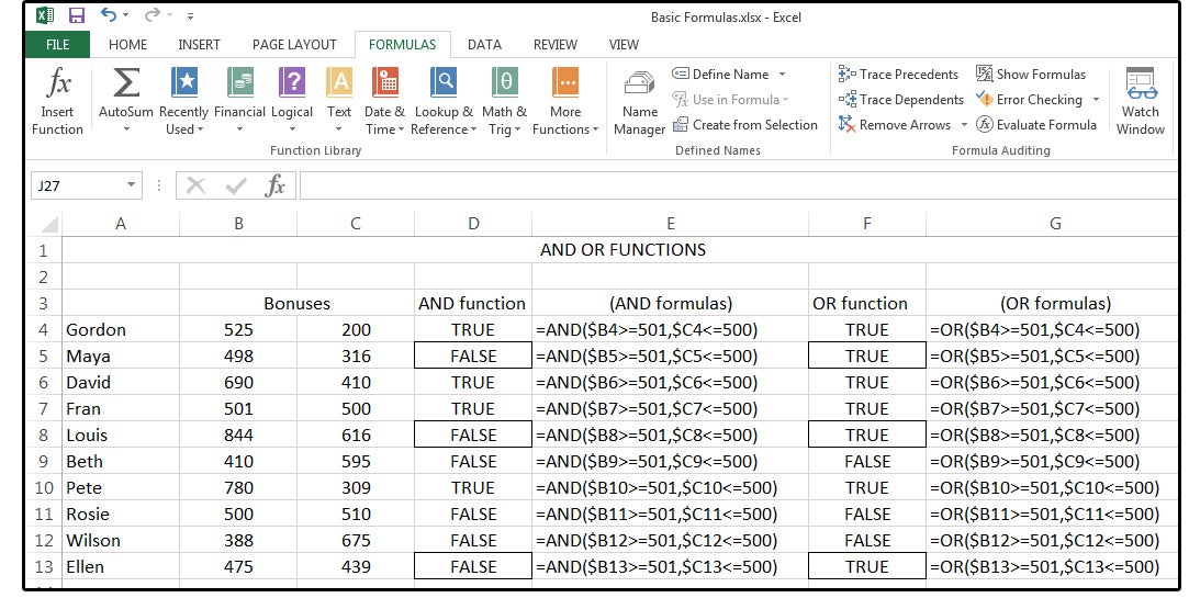
12. AND/OR

AND and OR are common functions in the programmers’ environment, also referred to as Boolean operators (along with NOT). AND means that all conditions in the query must be true; OR means that at least one condition must be true.
For example, looking for an applicant with MS Word AND MS Excel experience means the applicant must have both skills to qualify for the job. This condition would provide a TRUE result. Looking for an applicant with MS Word OR Excel means the applicant must have one OR the other, but not necessarily both. Also a TRUE result. Having neither skills would, obviously, provide a FALSE result.

1. Copy the numbers from the spreadsheet in figure 13, or download the full workbook (link below).
2. Enter the following AND formula in cell D4: =AND($B4>=501,$C4<=500). Again, note the $ signs. Then copy down to cell D13.
3. Enter this formula in cell F4: =OR($B4>=501,$C4<=500), then copy down. Notice the results in the rows with borders; that is, 5, 8, and 13. The AND results are all FALSE because both conditions were false (or not true); while the OR results were all TRUE because one of the conditions was true, while the other was false.

If this seems confusing, study the numbers in columns B and C. Then read the formulas that calculate for the AND function, then the OR function, and it will make more sense.


Source:
Indirabali